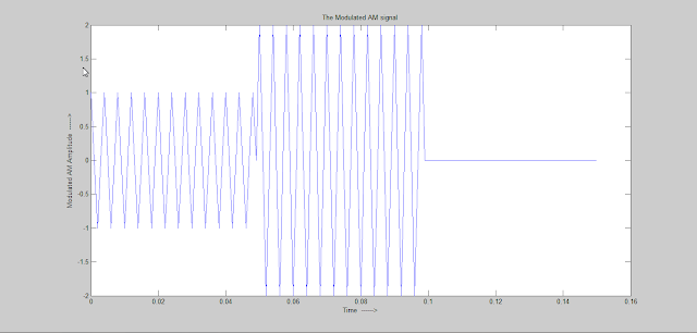
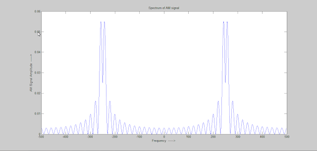
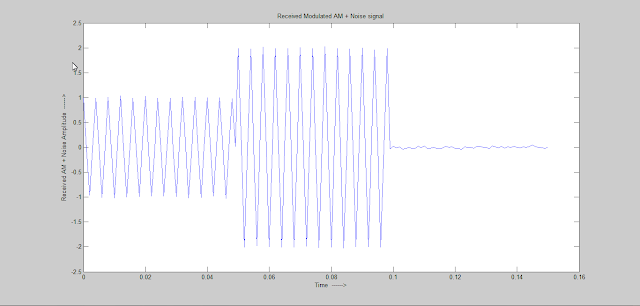
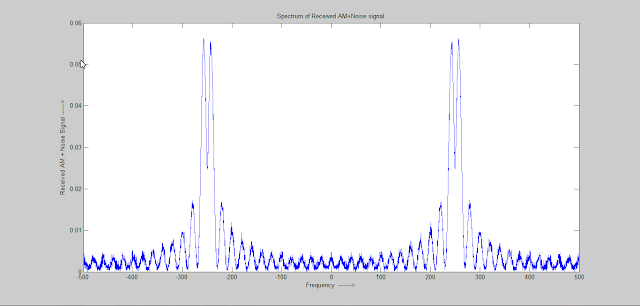
This article illustrates AM(Amplitude Modulation) in Matlab. Here the message signal m(t) consist of a rectangular pulse with +1 with 0.05 second duration and -2 amplitude pulse with duration of 0.05 second. This message signal modulates a carrier signal of 250Hz frequency to produce a DSB-AM signal. This transmitted DSB-AM signal s(t) is contaminated with noise n(t) in the channel. The received signal r(t) is thus s(t)+n(t). The SNR is assumed to be 20dB and a sampling frequency of 1KHz is used.
Running the AMmod.m matlab script provided below produces the various signal waveform and spectrum shown below. It also calculates the signal power and noise power for give SNR. The calculated signal power is 30.5mW and noise power is 0.30mW. The code uses the fftseq function that is also provided below.
For more tutorials see Video Tutorials and Matlab Tutorials
Let's Begin
The message signal is as follows-
\[m(t)=\begin{cases}+1 & 0\leq t \leq0.05\\-2 & 0.05\leq t \leq 0.1 \\ \space\space\space 0& \space\space otherwise\end{cases}\]
The waveform of this message signal is shown below-
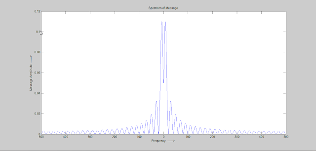
The corresponding Spectrum of the Message is shown below-
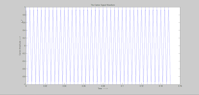
The Carrier signal is-
\[c(t)=cos(2\pi f_ct)\]
The Carrier waveform of frequency 250Hz is shown below-
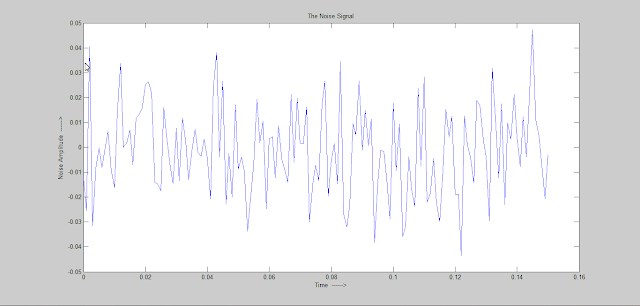
The noise signal waveform is shown below-
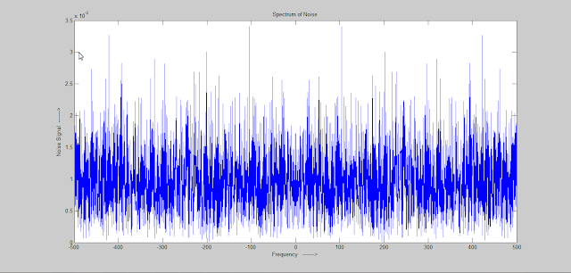
The Noise Spectrum is shown below-
The DSB-AM modulated wave equation is-
\[s(t)=m(t)*cos(2\pi f_ct)\]
The DSB-AM waveform is shown below-
The DSB-AM signal spectrum is shown below-
The received signal is-
\[r(t)=m(t)+n(t)\]
The waveform of this noise contaminated received signal is shown below-
The Spectrum of noise contaminated received signal is shown below-
Matlab Code
AMmod.m
----------------------------------------------------------------------------------------------------------------------
%Matlab Code for AM modulation Demonstration
to=0.05;
fs=1000;
ts=1/fs;
fc=250; %Carrier frequency
SNR_dB=20;
SNR_Linear=10^(SNR_dB/10);
df=0.3;
t=0:ts:3*to;
m=[ones(1,to/ts), -2*ones(1,to/ts), zeros(1,to/ts+1)]; %Message Signal
c=cos(2*pi*fc*t); %Carrier Signal
s=m.*c; %DSB-AM Signal
[M,m,df1]=fftseq(m,ts,df);
M=M/fs;
[C,c,df1]=fftseq(c,ts,df);
[S,s,df1]=fftseq(s,ts,df);
S=S/fs;
f=[0:df1:df1*(length(m)-1)]-fs/2; %frequency axis setting
message_power= (norm(m)^2)/length(m);
signal_power=(norm(s)^2)/length(s)
noise_power=signal_power/SNR_Linear;
noise_std=sqrt(noise_power);
n=noise_std*randn(1,length(s));
[N,n,df1]=fftseq(n,ts,df);
N=N/fs;
r=s+n;
[R,r,df1]=fftseq(r,ts,df);
R=R/fs;
pause
signal_power
pause
noise_power
pause
clf
figure %Message
plot(t,m(1:length(t)))
xlabel('Time ------>')
ylabel('Message Amplitude ----->')
title('The Message Signal Waveform')
pause
figure %Message
plot(t,c(1:length(t)))
xlabel('Time ------>')
ylabel('Carrier Amplitude ----->')
title('The Carrier Signal Waveform')
pause
figure %Noise
plot(t,n(1:length(t)))
xlabel('Time ------>')
ylabel('Noise Amplitude ------>')
title('The Noise Signal')
pause
figure %AM signal
plot(t,s(1:length(t)))
xlabel('Time ------>')
ylabel('Modulated AM Amplitude ------>')
title('The Modulated AM signal')
pause
figure %Received Signal
plot(t,r(1:length(t)))
xlabel('Time ------>')
ylabel('Received AM + Noise Amplitude ------>')
title('Received Modulated AM + Noise signal')
pause
figure %Message Spectrum
plot(f,abs(fftshift(M)))
xlabel('Frequency ------>')
ylabel('Message Amplitude ------>')
title('Spectrum of Message')
pause
figure %AM signal Spectrum
plot(f,abs(fftshift(S)))
xlabel('Frequency ------>')
ylabel('AM Signal Amplitude ------>')
title('Spectrum of AM signal')
pause
figure %Noise Spectrum
plot(f,abs(fftshift(N)))
xlabel('Frequency ------->')
ylabel('Noise Signal ------->')
title('Spectrum of Noise')
pause
figure %Received Signal Spectrum
plot(f,abs(fftshift(R)))
xlabel('Frequency ------->')
ylabel('Received AM + Noise Signal ------>')
title('Spectrum of Received AM+Noise signal')
---------------------------------------------------------------------------------------------------------------------
fftseq.m
---------------------------------------------------------------------------------------------------------------------
function [M,m,df]=fftseq(m,ts,df)
% [M,m,df]=fftseq(m,ts,df)
% [M,m,df]=fftseq(m,ts)
%FFTSEQ generates M, the FFT of the sequence m.
% The sequence is zero padded to meet the required frequency resolution df.
% ts is the sampling interval. The output df is the final frequency resolution.
% Output m is the zero padded version of input m. M is the FFT.
fs=1/ts;
if nargin == 2
n1=0;
else
n1=fs/df;
end
n2=length(m);
n=2^(max(nextpow2(n1),nextpow2(n2)));
M=fft(m,n);
m=[m,zeros(1,n-n2)];
df=fs/n;
-------------------------------------------------------------------------------------------------------------------------
See Download Matlab 2013 software
Running the AMmod.m matlab script provided below produces the various signal waveform and spectrum shown below. It also calculates the signal power and noise power for give SNR. The calculated signal power is 30.5mW and noise power is 0.30mW. The code uses the fftseq function that is also provided below.
For more tutorials see Video Tutorials and Matlab Tutorials
Let's Begin
The message signal is as follows-
\[m(t)=\begin{cases}+1 & 0\leq t \leq0.05\\-2 & 0.05\leq t \leq 0.1 \\ \space\space\space 0& \space\space otherwise\end{cases}\]
The waveform of this message signal is shown below-
 |
| Message Signal |
 |
| Message Signal Spectrum |
\[c(t)=cos(2\pi f_ct)\]
The Carrier waveform of frequency 250Hz is shown below-
 |
| Carrier signal waveform |
 |
| Noise |
 |
| Noise Spectrum |
\[s(t)=m(t)*cos(2\pi f_ct)\]
The DSB-AM waveform is shown below-
 |
| AM waveform |
 |
| AM Frequency Spectrum |
\[r(t)=m(t)+n(t)\]
The waveform of this noise contaminated received signal is shown below-
 |
| Noise contaminated AM modulated signal |
 |
| Noise Contaminated Received Signal Frequency Spectrum |
AMmod.m
----------------------------------------------------------------------------------------------------------------------
%Matlab Code for AM modulation Demonstration
to=0.05;
fs=1000;
ts=1/fs;
fc=250; %Carrier frequency
SNR_dB=20;
SNR_Linear=10^(SNR_dB/10);
df=0.3;
t=0:ts:3*to;
m=[ones(1,to/ts), -2*ones(1,to/ts), zeros(1,to/ts+1)]; %Message Signal
c=cos(2*pi*fc*t); %Carrier Signal
s=m.*c; %DSB-AM Signal
[M,m,df1]=fftseq(m,ts,df);
M=M/fs;
[C,c,df1]=fftseq(c,ts,df);
[S,s,df1]=fftseq(s,ts,df);
S=S/fs;
f=[0:df1:df1*(length(m)-1)]-fs/2; %frequency axis setting
message_power= (norm(m)^2)/length(m);
signal_power=(norm(s)^2)/length(s)
noise_power=signal_power/SNR_Linear;
noise_std=sqrt(noise_power);
n=noise_std*randn(1,length(s));
[N,n,df1]=fftseq(n,ts,df);
N=N/fs;
r=s+n;
[R,r,df1]=fftseq(r,ts,df);
R=R/fs;
pause
signal_power
pause
noise_power
pause
clf
figure %Message
plot(t,m(1:length(t)))
xlabel('Time ------>')
ylabel('Message Amplitude ----->')
title('The Message Signal Waveform')
pause
figure %Message
plot(t,c(1:length(t)))
xlabel('Time ------>')
ylabel('Carrier Amplitude ----->')
title('The Carrier Signal Waveform')
pause
figure %Noise
plot(t,n(1:length(t)))
xlabel('Time ------>')
ylabel('Noise Amplitude ------>')
title('The Noise Signal')
pause
figure %AM signal
plot(t,s(1:length(t)))
xlabel('Time ------>')
ylabel('Modulated AM Amplitude ------>')
title('The Modulated AM signal')
pause
figure %Received Signal
plot(t,r(1:length(t)))
xlabel('Time ------>')
ylabel('Received AM + Noise Amplitude ------>')
title('Received Modulated AM + Noise signal')
pause
figure %Message Spectrum
plot(f,abs(fftshift(M)))
xlabel('Frequency ------>')
ylabel('Message Amplitude ------>')
title('Spectrum of Message')
pause
figure %AM signal Spectrum
plot(f,abs(fftshift(S)))
xlabel('Frequency ------>')
ylabel('AM Signal Amplitude ------>')
title('Spectrum of AM signal')
pause
figure %Noise Spectrum
plot(f,abs(fftshift(N)))
xlabel('Frequency ------->')
ylabel('Noise Signal ------->')
title('Spectrum of Noise')
pause
figure %Received Signal Spectrum
plot(f,abs(fftshift(R)))
xlabel('Frequency ------->')
ylabel('Received AM + Noise Signal ------>')
title('Spectrum of Received AM+Noise signal')
---------------------------------------------------------------------------------------------------------------------
fftseq.m
---------------------------------------------------------------------------------------------------------------------
function [M,m,df]=fftseq(m,ts,df)
% [M,m,df]=fftseq(m,ts,df)
% [M,m,df]=fftseq(m,ts)
%FFTSEQ generates M, the FFT of the sequence m.
% The sequence is zero padded to meet the required frequency resolution df.
% ts is the sampling interval. The output df is the final frequency resolution.
% Output m is the zero padded version of input m. M is the FFT.
fs=1/ts;
if nargin == 2
n1=0;
else
n1=fs/df;
end
n2=length(m);
n=2^(max(nextpow2(n1),nextpow2(n2)));
M=fft(m,n);
m=[m,zeros(1,n-n2)];
df=fs/n;
-------------------------------------------------------------------------------------------------------------------------
See Download Matlab 2013 software
Tidak ada komentar:
Posting Komentar