Binary Block Encoding in Matlab

In Binary Block Encoding binary message are encoded in blocks of length k into codewords of length n. Here an illustration of C(6,3) block encoding is provided using Matlab. In the illustrating first binary message signal is defined then codewords are generated using a generator matrix. Errors are added to the encoded blocks to generated corrupted codewords and finally syndrome is calculated using the error vectors and received signal vectors. The syndrome with both the vectors are the same.

Let suppose we have binary message as follows-

m1=[0 0 0];
m2=[1 0 0];
m3=[0 1 0];
m4=[1 1 0];
m5=[0 0 1];
m6=[1 0 1];
m7=[0 1 1];
m8=[1 1 1];

The actual stream of message is- m=[m1 m2 m3 m4 m5 m6 m7 m8]

The codewords C{c1,c2,c3,c4,c5,c6} are generated by multiplying the Generator with the message blocks. Thus we need the generator block first. Let it be defined as follows-

G=[1 1 0 1 0 0; 0 1 1 0 1 0;1 0 1 0 0 1];

The the codewords is generated using the equation-

C=m*G

The matlab code that does this is-

c1=mod(double(m1)*double(G),2);
c2=mod(double(m2)*double(G),2);
c3=mod(double(m3)*double(G),2);
c4=mod(double(m4)*double(G),2);
c5=mod(double(m5)*double(G),2);
c6=mod(double(m6)*double(G),2);
c7=mod(double(m7)*double(G),2);
c8=mod(double(m8)*double(G),2);
 
The actual binary stream is C=[c1 c2 c3 c4 c5 c6 c7]. This encoded binary stream is modulated and transmitted over the noisy channel to the receiver. The received signal is demodulated and then sampled to get a binary received signal as follows-

r=c+e

where e=e1...e6 are errors introduced by the channel and added to the codewords. The errors are random and the codes for these errors are-

e1=round(rand(1,6));
e2=round(rand(1,6));
e3=round(rand(1,6));
e4=round(rand(1,6));
e5=round(rand(1,6));
e6=round(rand(1,6));

These errors are added to the transmitted codewords and the matlab code for the received binary bits are-

r1 = bsxfun(@plus,c1,e1);
r2 = bsxfun(@plus,c2,e2);
r3 = bsxfun(@plus,c3,e3);
r4 = bsxfun(@plus,c4,e4);
r5 = bsxfun(@plus,c5,e5);
r6 = bsxfun(@plus,c6,e6);

Once we have the received noise corrupted codewords we want to determine where and which bit is in error and correct the error bit if possible. To do this we can use Syndrome parameter. This parameter can be determined using two methods as follows-

S=r*H'
or
S=e*H'

Here H' is the transpose of a matrix H called the parity check matrix. The H matrix can be found out from the generator matrix by requiring that-

G*H'=0

Matlab has a special function called gentopar( ) that calculates the Parity check matrix from the Generator Matrix-

H=gen2par(G);

Once we know H and r(or e) we can determine the Syndrome. The two methods to calculate Syndrome gives the same value of syndrome(that is either using r or e). The matlab code for this is-

Sr1=mod(double(r1)*double(H'),2);
Sr2=mod(double(r2)*double(H'),2);
Sr3=mod(double(r3)*double(H'),2);
Sr4=mod(double(r4)*double(H'),2);
Sr5=mod(double(r5)*double(H'),2);
Sr6=mod(double(r6)*double(H'),2);

and,

Se1=mod(double(e1)*double(H'),2);
Se2=mod(double(e2)*double(H'),2);
Se3=mod(double(e3)*double(H'),2);
Se4=mod(double(e4)*double(H'),2);
Se5=mod(double(e5)*double(H'),2);
Se6=mod(double(e6)*double(H'),2);

We can check that the Syndrome calculated using received vector r and error vector e are the same. That is for example Sr5 and Se5 are the same or Sr2 and Se2 are the same and likewise others.

A Syndrome of all zero vector implies no error and a non-zero vector implies error. For example the following Matlab code outputs syndrome of Sr2 = [0 1 1] showing that there are errors.

-------------------------------------------------------------------------------------------------------------------
Complete Matlab Code
 -------------------------------------------------------------------------------------------------------------------
% Block Encoding Decoding for (6,3)

clear all;
clc

% Define block of message sequences

m1=[0 0 0];
m2=[1 0 0];
m3=[0 1 0];
m4=[1 1 0];
m5=[0 0 1];
m6=[1 0 1];
m7=[0 1 1];
m8=[1 1 1];

m=[m1 m2 m3 m4 m5 m6 m7 m8];

% Define Generator matrix G

G=[1 1 0 1 0 0; 0 1 1 0 1 0;1 0 1 0 0 1];

%Generate Codewords C

c1=mod(double(m1)*double(G),2);
c2=mod(double(m2)*double(G),2);
c3=mod(double(m3)*double(G),2);
c4=mod(double(m4)*double(G),2);
c5=mod(double(m5)*double(G),2);
c6=mod(double(m6)*double(G),2);
c7=mod(double(m7)*double(G),2);
c8=mod(double(m8)*double(G),2);



% Define Noise

e1=round(rand(1,6));
e2=round(rand(1,6));
e3=round(rand(1,6));
e4=round(rand(1,6));
e5=round(rand(1,6));
e6=round(rand(1,6));

% Generate Received Signal with Noise

r1 = bsxfun(@plus,c1,e1);
r2 = bsxfun(@plus,c2,e2);
r3 = bsxfun(@plus,c3,e3);
r4 = bsxfun(@plus,c4,e4);
r5 = bsxfun(@plus,c5,e5);
r6 = bsxfun(@plus,c6,e6);

% Generate Parity check Matrix H

H=gen2par(G);

% Generate Syndrome using r vectors

Sr1=mod(double(r1)*double(H'),2);
Sr2=mod(double(r2)*double(H'),2);
Sr3=mod(double(r3)*double(H'),2);
Sr4=mod(double(r4)*double(H'),2);
Sr5=mod(double(r5)*double(H'),2);
Sr6=mod(double(r6)*double(H'),2);

% Generate Syndrome using e vectors

Se1=mod(double(e1)*double(H'),2);
Se2=mod(double(e2)*double(H'),2);
Se3=mod(double(e3)*double(H'),2);
Se4=mod(double(e4)*double(H'),2);
Se5=mod(double(e5)*double(H'),2);
Se6=mod(double(e6)*double(H'),2);

-------------------------------------------------------------------------------------------------------------------

Labview Tutorial on Analog Modulation

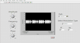
This Labview tutorial demonstrates AM, FM and PM analog modulation using real audio signal contained in .wav file. An interface is constructed that allows users to choose the different modulation and also allows to vary the amplitude, frequency, phase, frequency modulation index and phase modulation index.

Before we start you might want to visit Labview Student Download and Labview Tutorials.

The complete front panel view and the back progamming panel are shown below-

Figure 1: Modulation Labview Front Panel View

Figure 2: Modulation Labview Back Program View

Basically this program allows us to browse and select an audio file in the .wav format which is then amplitude modulated or frequency modulated or phase modulated according to what users chooses from the modulation selector(see figure 1). If freqency modulation or phase modulation is selected then users can input the freqeuncy modulation index or phase modulation index respectively. There are also three numeric controls for amplitude, frequency and phase. For audio file input control use the file path control which can be found in modern, silver and also in the classic control pallet of the front control panel.

The back programming panel consist mainly of numeric inputs(amplitude,frequency,phase, index constants), the file importing function element, three formula nodes, a case structure, a waveform chart, timer and stop. All these functional elements are embedded inside the while loop.

The carrier and audio signal inputs enters the three AM, FM and PM formula nodes and each outputs the different modulated signals. The case structure allows to select which modulated signal to plot on the waveform chart. 

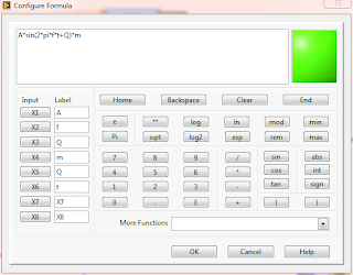
The figure below shows how the formula for AM, FM and PM is written into the formula node-

Figure 3: AM formula node in Labview

In the above AM formula, A is the amplitude, f the frequency, t the time, Q the phase and m the audio signal(message). Note that the time t is obtained from the iteration index number of the while loop.

Similarly the FM formula node is-

Figure 4: FM formula node in Labview

In this case, kf is the frequency modulation index, int(m) is the integration of the audio signal and others are same as for the AM signal formula.

Lastly the PM formula node is-

Figure 5: PM formula node in Labiview

Here kf is the phase modulation index.

An introduction tutorial of Labview

This is an introduction tutorial on Labview which shows how to use enter the input and output controls into the front panel and the functional parts in the block diagram panel. After having placed the required controls and elements we perform simulation to get output.

Readers may acquire Labview download student, visit the blog post.

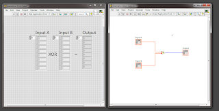
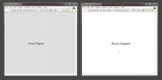
The Labview can consist of two panel- Front Panel and Block Diagram Panel. The front panel is used to place users input/output controls blocks and the block diagram panel is where you put the the actual algorithm implementation using functional blocks.

The picture below shows these two panels-

Picture: Labview front and block diagram panel

Here we give an simple example on how to set up labview to perform XOR of two sequence of binary data sequence.

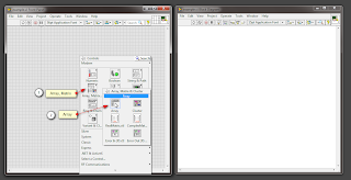
To do this right click on the Front panel and select Array,Matrix & Cluster then Array as shown

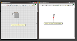
Once it is single clicked it is attached automatically attached to the mouse cursor. Place the input array in suitable location in the front panel workspace. As it is placed on the front panel the corresponding functional block is added in the block diagram panel as shown-

Now place another two such arrays-

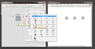
Now to define input and output we have to place numeric input and output(indicator) inside the array. To do this, right click and select Numeric>Numeric Control as shown below and drop it inside the first array box.

Now drag the array so that it has 8 rows-

Repeat the same process for Array2.

For the Array3 we need to insert Numeric Indicator instead of Numeric Control because it is the output . Insert the Numeric Indicator into the Array3 as shown-

Change the labels Array, Array2 and Array3 by simple double clicking it and editing to Input A, Input B and Output.

To make more descriptive on what the inputs are doing to get the output, just double click on the space between Input A and Input B and write 'XOR' and write a '=' between the Input B and Output array as shown below. Note that you can increase the Font size using ctrl+=.

We are finished for now with the input/output interface design. Now we will have to add the function XOR in the block diagram panel.

To do this relocate the array blocks in the block diagram that looks something like the one below-

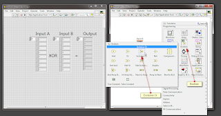
Now right click on the block diagram panel and add the XOR by going to Boolean>Exclusive Or as shown below-

The picture below shows the XOR block in between the input and output-

Now join them with the wires as shown-

Now the entry step is complete and we need to run the simulation. But before running the simulation we need to add the binary digits into the Input A and Input B array in the Front Panel. Enter random binary digits. The following shows an example-

Notice that the output is grayed colored.

Now we are ready for simulation. Click on the 'Run Continuously' icon on the toolbar and we get the output result. This is shown below-

The XOR outputs 0 when both inputs are 1 or 0 and outputs 1 when the inputs are different. As seen from the output the output is XOR of the inputs.

This completes the introduction tutorial of Labview.

Power Spectral Density of Polar Signals

Last time we discussed about the power spectral density of NRZ and RZ On-Off signal. This article is a continuation of power spectral densities of line coders and here PSD of NRZ and RZ polar signal will be plotted with Matlab.

We start with the definition of NRZ and RZ polar signal with mathematical formula and then plot the PSD of those signals.

For definition see Energy Spectral Density and Power Spectral Density blog post.

NRZ Polar Signal

A Polar signal is one in which binary one is represented by a +ve pulse and binary zero is represented by a -ve pulse. A NRZ(Non-Return-Zero) polar signal is one in which the bits(i.e the +ve and -ve pulse) has a full width duration called the bit duration or pulse duration.

An example of a binary sequence 100 in NRZ polar form is shown below-

Figure: example of polar NRZ sequence

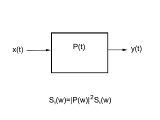
Now we wish to calculate the power spectral density of such signal. That is looking at the figure below we wish to calculate the power spectral density of the output signal y(t).

Figure: PSD input output relation

In order to calculate Sy(w) and to do this we need Sx(w) and P(w), see equation below-
\[S_y(w)=|P(w)|^{2}S_x(w)\space\space\space\space\space\space---->(1)\]
For a NRZ rectangular polar signals as shown above the Fourier Transform P(w) of such signal is-
 \[P(w)=T_b*sinc(\frac{w*T_b}{2})\space\space\space\space\space\space\space\space\space\space\space\space------>(2)\]
The derivation of final PSD Sx(w) of input signal x(t) is lengthy and we provide only the final result. The PSD Sx(w) is-
\[S_x(w)=\frac{1}{T_b}(R_0+2\sum_{n=1}^\infty R_ncos(nwT_b))\]
Determining the autocorrelation we find that Ro=1 and Rn=0 and the above equation simplifies to-
\[S_x(w)=\frac{1}{T_b}\space\space\space\space\space\space\space\space\space\space\space------>(3)\]
Using the equation (2) and (3) result in equation (1), the PSD Sy(w) is-
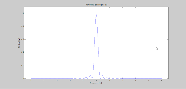
\[S_y(w)=T_b*sinc^{2}(\frac{{w*T_b}}{2})\space\space\space\space\space\space\space\space\space\space\space------>(4)\]

The matlab code to generate this PSD is below-

% Generates PSD of NRZ polar signal

clear on
clc

Tb=1;
Rb=1/Tb;
faxis=-5*Rb:Rb/100:5*Rb;
w=2*pi*faxis;
Sy=Tb*(sinc((w*Tb)/2)).^2
plot(faxis,Sy)
xlabel('Frequency(Hz)')
ylabel('PSD (W/Hz)')
title('PSD of NRZ polar signal y(t)')
axis([-5.5 5.5 -0.01 1.1])

The plot is shown below-

Figure: Power spectral density of NRZ polar signal

RZ Polar Signal
A RZ polar signal is one in which the pulses representing the binary bits 1 and 0 has a half width bit duration or pulse duration. This is illustrated in the picture below-

Figure: RZ polar signal

Again visualizing the input/output PSD relation as shown in picture above and the equation (1) we require the Px(w) and Sx(w) for this RZ polar signal.

The Fourier transform of RZ polar pulse is-
 \[P(w)=\frac{T_b}{2}*sinc(\frac{w*T_b}{4})\space\space\space\space\space\space\space\space\space\space\space\space------>(5)\]
 And the PSD of the input signal is-
\[S_x(w)=\frac{1}{T_b}\space\space\space\space\space\space\space\space\space\space\space------>(6)\]
Thus using equation (5) and (6) in equation (1) we get-
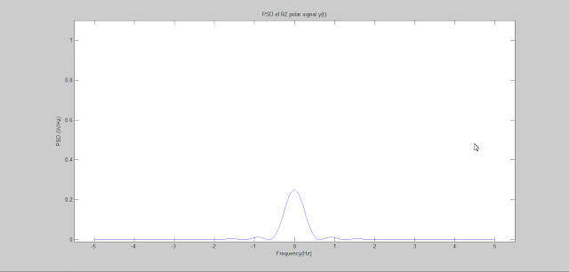
\[S_y(w)=\frac{T_b}{4}*sinc^{2}(\frac{{w*T_b}}{4})\space\space\space\space\space\space\space\space\space\space\space------>(7)\]

The matlab for this PSD is below-

% Generates PSD of RZ polar signal

clear on
clc

Tb=1;
Rb=1/Tb;
faxis=-5*Rb:Rb/100:5*Rb;
w=2*pi*faxis;
Sy=(Tb/4)*(sinc((w*Tb)/4)).^2
plot(faxis,Sy)
xlabel('Frequency(Hz)')
ylabel('PSD (W/Hz)')
title('PSD of RZ polar signal y(t)')
axis([-5.5 5.5 -0.01 1.1])

The plot is shown below-

Figure: Power Spectral Density of RZ polar signal

See more Matlab Tutorials
 

Power Spectral Density of On-Of signalling

This tutorial is about Power Spectral Density(PSD) of NRZ and RZ On-Off signals using Matlab. We start with definition and derivation of PSD for each and then generate the matlab code to plot the spectral densities. In the next tutorial we will plot PSD of Polar signals.

Readers interested in circuit simulation in orcad capture of such baseband encoding can visit the following tutorials here on this blog-

• AMI Bipolar Encoding
• NRZ Unipolar and Bipolar Encoding

In the communication system design and engineering, Power spectral density is an important parameter as it gives us the information about the Power contained by a signal. This in turn gives us indication about SNR and thereof the distance between the transmitter and the receiver among many other things.

Suppose x(t) is an input signal that goes into a pulse shaping filter with response p(t) and the output of the pulse shaping filter is y(t). Let their respective Fourier Transform be X(w), P(w) and Y(w)respectively and their the PSD of x(t) and PSD of y(t) be Sx(w) and Sy(w). This concept is shown below-

Then the relation between input and output PSD is-                       \[S_y(w)=|P(w)|^{2}S_x(w)\space\space\space\space\space\space---->(1)\]
Hence to find out the PSD of the output signal y(t) we require two things- the PSD of the input signal x(t) and the F.T. P(w) of the pulse p(t).

For each NRZ and RZ On-Off signal both Sx(w) and P(w) will be different. We show the values of these parameters starting with NRZ and then for RZ.

NRZ On-Off Signalling

In case of NRZ, binary one is transmitted using a +ve pulse p(t) for full bit duration Tb and binary zero is transmitted by transmitting nothing. The diagram for NRZ On-Off signal is shown is shown below-

Figure: NRZ On Off Signal

This rectangular signal is defined as-
\[p(t)=rect(t/T)=\begin{cases}1 & -T_b/2< t < T_b/2\\0 & \space\space\space\space\space\space\space\space\space\space\space|t|>1/2\end{cases}\]
The FT of this signal is
\[P(w)=\int_{0}^{T_b} p(t)*e^{-jwt} dt=\int_{-T_b/2}^{T_b/2} p(t)*e^{-jwt} dt=\int_{-T_b/2}^{T_b/2} e^{-jwt} dt\]
This evaluates to,
\[P(w)=T_b*sinc(\frac{w*T_b}{2})\space\space\space\space\space\space\space\space\space\space\space\space------>(2)\]
The derivation of PSD of x(t) is lengthy so we directly show it here. The PSD of x(t) is given by-
\[S_x(w)=\frac{1}{4*T_b}+\frac{2\pi}{4*T_b^{2}}\sum_{n=-\infty}^\infty\delta(w-\frac{2\pi n}{T_b})\space\space\space\space\space\space---->(3)\]
From equation (1) using equation (2) and (3), the PSD of output signal y(t) evaluates to-
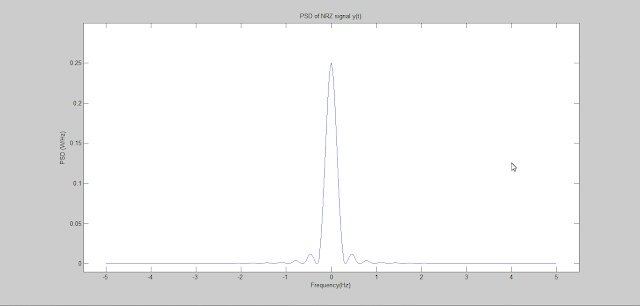
\[S_y(w)=\frac{T_b}{4}*sinc^{2}(\frac{w*T_b}{2})+\frac{\pi}{2}\delta(w) \space\space\space\space\space\space---->(4)\]

The matlab code to generate this PSD is provided below-

% PSD of On-Off NRZ signal
clear on
clc

Tb=1;
Rb=1/Tb;
faxis=-5*Rb:Rb/100:5*Rb;
w=2*pi*faxis;
Sy=(Tb/4)*(sinc((w*Tb)/2)).^2
plot(faxis,Sy)
xlabel('Frequency(Hz)')
ylabel('PSD (W/Hz)')
title('PSD of NRZ signal y(t)')
axis([-5.5 5.5 -0.01 0.3])

The Power spectral density of NRZ On-Off signal is shown below-

Figure: Power spectral density of NRZ On-Off signalling

RZ On-Off Signalling

A rectangular RZ On-Off signal is shown below-

Figure: RZ On Off Signal

As seen from the figure the pulse for binary one has a bit duration of Tb/2.

This rectangular signal is defined as-
\[p(t)=rect(2t/T)=\begin{cases}1 & -T_b/4< t < T_b/4\\0 & \space\space\space\space\space\space\space\space\space\space\space|t|>1/4\end{cases}\]
The FT of this signal is
\[P(w)=\int_{0}^{T_b/2} p(t)*e^{-jwt} dt=\int_{-T_b/4}^{T_b/4} p(t)*e^{-jwt} dt=\int_{-T_b/4}^{T_b/4} e^{-jwt} dt\]
This evaluates to,
\[P(w)=\frac{T_b}{2}*sinc(\frac{w*T_b}{4})\space\space\space\space\space\space\space\space\space\space\space\space------>(5)\]
Again PSD of x(t) will not be derived here. The PSD of x(t) is given by-
\[S_x(w)=\frac{1}{4*T_b}+\frac{2\pi}{4*T_b^{2}}\sum_{n=-\infty}^\infty\delta(w-\frac{2\pi n}{T_b})\space\space\space\space\space\space---->(6)\]
Substituting equation (5) and (6) into equation (1) yields the PSD of output signal y(t) as-
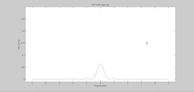
\[S_y(w)=\frac{T_b^{2}}{16}*sinc^{2}(\frac{w*T_b}{4})[1+\frac{2 \pi}{T_b}\sum_{n=-\infty}^\infty\delta(w-\frac{2 \pi}{T_b})] \space\space\space\space\space\space---->(7)\]
 The matlab code to generate this PSD is provided below-

% PSD of ON-OFF RZ signal

Tb=1;
Rb=1/Tb;
faxis=-5*Rb:Rb/100:5*Rb;
w=2*pi*faxis;
Sy=(Tb^2/16)*sinc((w*Tb)/4).^2;
plot(faxis,Sy)
xlabel('Frequency(Hz)')
ylabel('PSD (W/Hz)')
title('PSD of RZ signal y(t)')
axis([-5.5 5.5 -0.01 0.3])

The PSD of RZ On-Off signal is shown below-

Figure: Power Spectral Density of RZ On-Off signal

See more Matlab tutorials 

QPSK signal generation in Matlab

QPSK modulation is a widely used digital modulation technique. It is a bandwidth efficient scheme because it allows to transmit two bits per symbol. Bandwidth efficient means that more information bits can be transmitted for a given allocated bandwidth. In this article the QPSK modulation is explained with the help of Matlab.

The mathematical form of QPSK signal is-

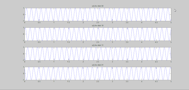
\[s(t)=\begin{cases}Acos(2\pi f_ct-\frac{3\pi}{4}) & dibit\space 00\\Acos(2\pi f_ct-\frac{\pi}{4}) & dibit\space10\\Acos(2\pi f_ct+\frac{\pi}{4}) & dibit\space01\\Acos(2\pi f_ct+\frac{3\pi}{4}) & dibit\space 11 \end{cases}\]

where, \[0\leq t\leq T\]  and T is the symbol duration

The QPSK signal can also be written in the following compact form-
\[s(t)=Acos(2\pi f_ct+\phi (t)) \]
where,
\[\phi(t)=\begin{cases}-\frac{3\pi}{4} & dibit\space00\\-\frac{\pi}{4} & dibit\space10\\+\frac{\pi}{4} & dibit\space01\\+\frac{3\pi}{4} & dibit\space11 \end{cases}\]
The matlab code to generate these four QPSK signal is below-

% Generation of QPSK signal

clear
echo on
Ac=1                    %Carrier Amplitude
fs=100;                    %Sampling frequency
fc=6;                    % carrier frequency               
t=0:1/fs:5;
s00=Ac*cos(2*pi*fc*t-(3*pi/4));       %QPSK for dibit 00
s10=Ac*cos(2*pi*fc*t-(pi/4));         %QPSK for dibit 10
s11=Ac*cos(2*pi*fc*t+(3*pi/4));       %QPSK for dibit 11
s01=Ac*cos(2*pi*fc*t+(pi/4));         %QPSK for dibit 01
% plotting commands follow
subplot(4,1,1);
plot(t,s00);
title('s(t) for dibit 00')
subplot(4,1,2);
plot(t,s10);
title('s(t) for dibit 10')
subplot(4,1,3);
plot(t,s11);
title('s(t) for dibit 11')
subplot(4,1,4);
plot(t,s01)
title('s(t) for dibit 01')

The QPSK signal graph is shown below-

QPSK signal waveform

 See more on Matlab Tutorials

PSK Modulation Simulation Video Tutorial

This video tutorial shows PSK modulation simulation using Orcad Capture software. The modulator is a Ring Modulator. The Message signal is in the form of binary sequences and fed into the secondary coil of the center tapped transformer of the modulator while the carrier signal is fed into the primary winding. At the other side of the ring modulator, PSK signal is generated. This is shown in graph plot.

<math xmlns='http://www.w3.org/1998/Math/MathML'><mrow><mrow><mi mathcolor='#0000ff' color='#0000ff' fontstyle='2D Output' fontweight='normal'>s</mi><mo>&ApplyFunction;</mo><mfenced open='(' close=')' separators=','><mrow><mi mathcolor='#0000ff' color='#0000ff' fontstyle='2D Output' fontweight='normal'>t</mi></mrow></mfenced></mrow><mo>&#x3d;</mo><mrow><mi mathcolor='#0000ff' color='#0000ff' fontstyle='2D Output' fontweight='normal'>A</mi><mo>&InvisibleTimes;</mo><mrow><mi mathcolor='#0000ff' mathvariant='normal' color='#0000ff' fontstyle='2D Output' fontweight='normal'>cos</mi><mo>&ApplyFunction;</mo><mfenced open='(' close=')' separators=','><mrow><mrow><mrow><mn mathcolor='#0000ff' color='#0000ff' fontstyle='2D Output' fontweight='normal'>2</mn><mo>&InvisibleTimes;</mo><mo>&InvisibleTimes;</mo><mi mathcolor='#0000ff' color='#0000ff' fontstyle='2D Output' fontweight='normal'>t</mi></mrow><mo>&#x2b;</mo><mfenced open='{' close='}' separators=','><mrow><mi mathcolor='#0000ff' color='#0000ff' fontstyle='2D Output' fontweight='normal'></mi></mrow></mfenced></mrow></mrow></mfenced></mrow></mrow></mrow></math>

AM modulation illustration in Matlab

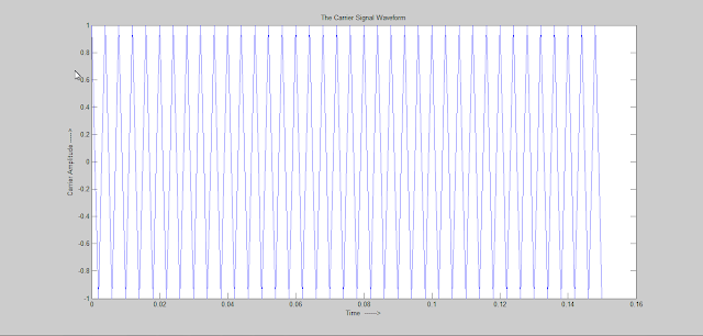
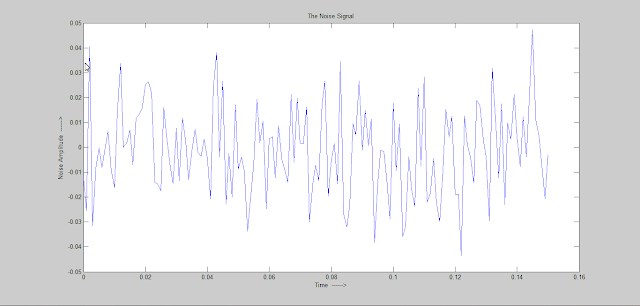
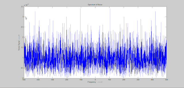
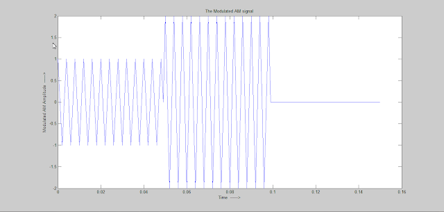
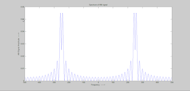
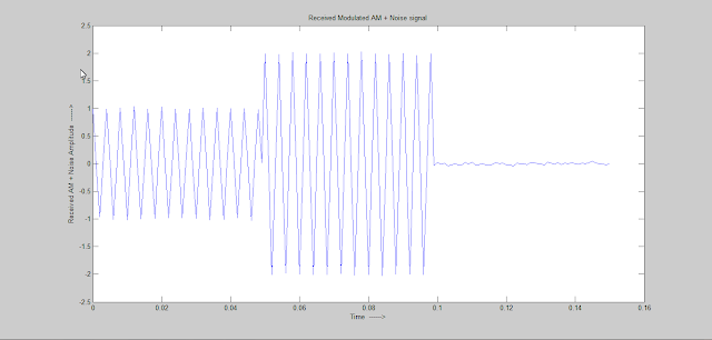
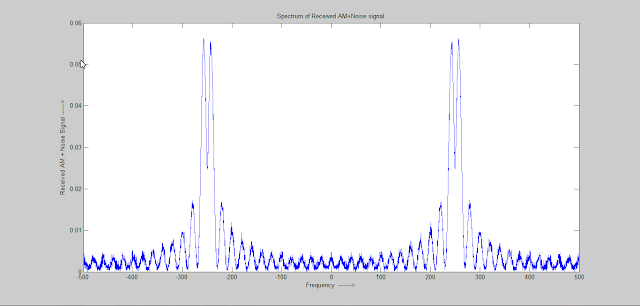
This article illustrates AM(Amplitude Modulation) in Matlab. Here the message signal m(t) consist of a rectangular pulse with +1 with 0.05 second duration and -2 amplitude pulse with duration of 0.05 second. This message signal modulates a carrier signal of 250Hz frequency to produce a DSB-AM signal. This transmitted DSB-AM signal s(t) is contaminated with noise n(t) in the channel. The received signal r(t) is thus s(t)+n(t). The SNR is assumed to be 20dB and a sampling frequency of 1KHz is used.

Running the AMmod.m matlab script provided below produces the various signal waveform and spectrum shown below. It also calculates the signal power and noise power for give SNR. The calculated signal power is 30.5mW and noise power is 0.30mW. The code uses the fftseq function that is also provided below.

For more tutorials see Video Tutorials and Matlab Tutorials

Let's Begin

The message signal is as follows-

\[m(t)=\begin{cases}+1 & 0\leq t \leq0.05\\-2 & 0.05\leq t \leq 0.1 \\ \space\space\space 0& \space\space otherwise\end{cases}\]

The waveform of this message signal is shown below-

Message Signal

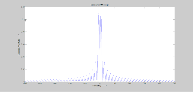
The corresponding Spectrum of the Message is shown below-

Message Signal Spectrum

 The Carrier signal is-
                      \[c(t)=cos(2\pi f_ct)\]
The Carrier waveform of frequency 250Hz is shown below-

Carrier signal waveform

 The noise signal waveform is shown below-

Noise

 The Noise Spectrum is shown below-

Noise Spectrum

The DSB-AM modulated wave equation is-
                      \[s(t)=m(t)*cos(2\pi f_ct)\]
The DSB-AM waveform is shown below-

AM waveform

 The DSB-AM signal spectrum is shown below-

AM Frequency Spectrum

 The received signal is-
                      \[r(t)=m(t)+n(t)\]
The waveform of this noise contaminated received signal is shown below-

Noise contaminated AM modulated signal

 The Spectrum of noise contaminated received signal is shown below-

Noise Contaminated Received Signal Frequency Spectrum

Matlab Code

AMmod.m
----------------------------------------------------------------------------------------------------------------------
%Matlab Code for AM modulation Demonstration
to=0.05;
fs=1000;
ts=1/fs;
fc=250;                                                            %Carrier frequency
SNR_dB=20;
SNR_Linear=10^(SNR_dB/10);
df=0.3;
t=0:ts:3*to;
m=[ones(1,to/ts), -2*ones(1,to/ts), zeros(1,to/ts+1)];               %Message Signal
c=cos(2*pi*fc*t);                                                    %Carrier Signal
s=m.*c;                                                              %DSB-AM Signal
[M,m,df1]=fftseq(m,ts,df);
M=M/fs;
[C,c,df1]=fftseq(c,ts,df);
[S,s,df1]=fftseq(s,ts,df);
S=S/fs;
f=[0:df1:df1*(length(m)-1)]-fs/2;                       %frequency axis setting
message_power= (norm(m)^2)/length(m);  
signal_power=(norm(s)^2)/length(s)
noise_power=signal_power/SNR_Linear;
noise_std=sqrt(noise_power);
n=noise_std*randn(1,length(s));
[N,n,df1]=fftseq(n,ts,df);
N=N/fs;
r=s+n;
[R,r,df1]=fftseq(r,ts,df);
R=R/fs;
pause
signal_power
pause
noise_power
pause
clf
figure                       %Message
plot(t,m(1:length(t)))
xlabel('Time  ------>')
ylabel('Message Amplitude ----->')
title('The Message Signal Waveform')
pause
figure                       %Message
plot(t,c(1:length(t)))
xlabel('Time  ------>')
ylabel('Carrier Amplitude ----->')
title('The Carrier Signal Waveform')
pause
figure                        %Noise
plot(t,n(1:length(t)))
xlabel('Time  ------>')
ylabel('Noise Amplitude  ------>')
title('The Noise Signal')
pause
figure                        %AM signal
plot(t,s(1:length(t)))
xlabel('Time  ------>')
ylabel('Modulated AM Amplitude  ------>')
title('The Modulated AM signal')
pause
figure                           %Received Signal
plot(t,r(1:length(t)))
xlabel('Time  ------>')
ylabel('Received AM + Noise Amplitude  ------>')
title('Received Modulated AM + Noise signal')
pause
figure                          %Message Spectrum
plot(f,abs(fftshift(M)))
xlabel('Frequency  ------>')
ylabel('Message Amplitude  ------>')
title('Spectrum of Message')
pause
figure                            %AM signal Spectrum
plot(f,abs(fftshift(S)))
xlabel('Frequency  ------>')
ylabel('AM Signal Amplitude  ------>')
title('Spectrum of AM signal')
pause
figure                               %Noise Spectrum
plot(f,abs(fftshift(N)))
xlabel('Frequency   ------->')
ylabel('Noise Signal  ------->')
title('Spectrum of Noise')
pause
figure                              %Received Signal Spectrum
plot(f,abs(fftshift(R)))
xlabel('Frequency  ------->')
ylabel('Received AM + Noise Signal ------>')
title('Spectrum of Received AM+Noise signal')
---------------------------------------------------------------------------------------------------------------------
fftseq.m
---------------------------------------------------------------------------------------------------------------------
function [M,m,df]=fftseq(m,ts,df)
%       [M,m,df]=fftseq(m,ts,df)
%       [M,m,df]=fftseq(m,ts)
%FFTSEQ     generates M, the FFT of the sequence m.
%       The sequence is zero padded to meet the required frequency resolution df.
%       ts is the sampling interval. The output df is the final frequency resolution.
%       Output m is the zero padded version of input m. M is the FFT.
fs=1/ts;
if nargin == 2
  n1=0;
else
  n1=fs/df;
end
n2=length(m);
n=2^(max(nextpow2(n1),nextpow2(n2)));
M=fft(m,n);
m=[m,zeros(1,n-n2)];
df=fs/n;
-------------------------------------------------------------------------------------------------------------------------

See Download Matlab 2013 software

Generation of Different Types of Signals in Matlab

In this article it is shown how to generate various important signals in Matlab. The different types of signal includes Unit Impulse, Unit Step, square, rectangle. sawtooth and others. In the study of communication system these signals appear frequently and thus knowledge about how to generate them in Matlab is important. For more see matlab tutorials and matlab software download.

Here we show the generation of following signals-

1. Unit Impulse signal
2. Unit Step signal
3. Signum signal
4. Square wave signal
5. Rectangular wave signal

1. Unit Impulse (Delta Function):

The dirac delta function (continuous and discrete)is defined as-
\[\delta(t)=\begin{cases}1 & t = 0\\0 & otherwise\end{cases}\]
or,

\[\delta(n)=\begin{cases}1 & n = 0\\0 & otherwise\end{cases}\]
To generate a unit Impulse the following matlab statement can be used-

>> Imp=[1 zeros(1,N-1)]

Let the number of zeros be N=8, then

>> Imp=[1 zeros(1,7)];

This creates a sequence- 1 0 0 0 0 0 0 0

Applying stem function-

>> stem(Imp)

gives the following graph-

Unit Impluse Sequence

To create shifted unit impulse we can use the following matlab statement-

>> Imp_shift= [zeros(1,k-1) 1 zeros(1,N-k)]

If N=8 and k=2,

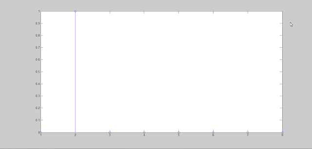
>> Imp_shift[zeros(1,1) 1 zeros(1,6)]

gives the sequence- 0 1 0 0 0 0 0 0

and,
>> stem(Imp_shift)

gives the following graph-

Shifted Unit Impulse

2. Unit Step Function

The unit step function is defined as-
 \[u(t)=\begin{cases}1 & t \geq 0\\0 & t < 0\end{cases}\]
or,
\[u(n)=\begin{cases}1 & n \geq 0\\0 & n < 0\end{cases}\]

To generate unit step sequence of length N the following matlab statement can be used-

u_step=[ones(1,N)]

let N=8, then we have

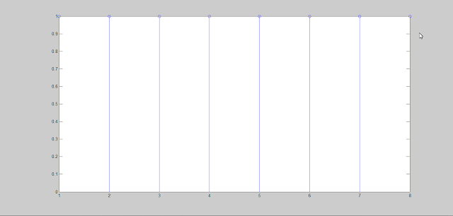
>> u_step=[ones(1,8)]

gives the sequence- 1 1 1 1 1 1 1 1

>> stem(u_step)

gives the following graph-

unit step sequence

Similarly, to generate a shifted unit step sequence u(n-k)we can use the following matlab statement-

u_step_shift=[zeros(1,k) ones(1,N)]

let N=8, k=3 then,

>> u_step_shift=[zeros(1,3) ones(1,8)]

gives the sequence-  0 0 0 1 1 1 1 1 1 1 1 (that is, three Zeros followed by eight Ones)

>> stem(u_step_shift)

gives the following graph-

shifted unit step sequence

Another method to generate unit step function is to use the heaviside(x) matlab function. The following command and graph illustrates generation of unit step function using this heaviside(x) command.

>> n = -5:0.01:5;
>> u_step = heaviside(n);
>> plot(n,u_step)

This gives the following graph-

unit step function using heaviside function

It's also easier to use heaviside function to generate a shifted unit step u(t-to) (or u(n-k)) as illustrated below-

>> n = -5:0.01:5;
>> u_step_shift = heaviside(n-2);
>> plot(n,u_step_shift)

shifted unit step function using heaviside function

3. Signum Function

The Signum function is defined as-

\[sign(t)=\begin{cases}1 & t< 0\\0 & t=0\\-1 & t>0\end{cases}\]
or,
\[sign(n)=\begin{cases}1 & n< 0\\0 & n=0\\-1 & n>0\end{cases}\]

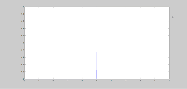
To generate the sign(n) function the matlab code is-

>> n=-5:0.01:5;
>> y=sign(n);
>> plot(n,y)

The graph is shown below-

Signum function

4. Square wave signal

Square signals can be generated using the square(t,duty) function. This function generates a periodic square wave with period T=2*pi with +ve and -ve unity peak value over the range defined by parameter t. The parameter duty defines percentage of period T over which the square wave remains positive.

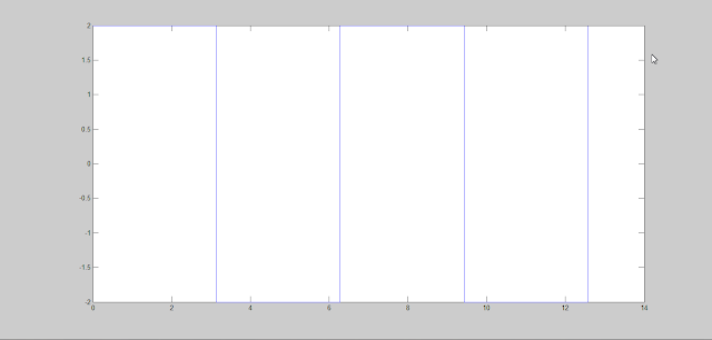
Example: To generate a square wave over two period 2T=4*pi and amplitude of 2

>> t=0:0.001*pi:4*pi;
>> y=2*square(t);
>> plot(t,y)

The plot is shown below-

Square wave signal

5. Rectangular wave signal

To generate rectangular signal in matlab we can use rectpuls(t) or rectpuls(t,w). rectpuls(t) function generates a continuous, aperiodic and unity height rectangular pulses. rectpuls(t,w) is same as rectpuls(t) with additional parameter w which allows to define width of the pulse.

Example:
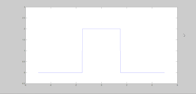
To generate a rectangular pulse of amplitude 2, pulse width 3 we use the following commands-

>> t=-5:0.01:5;
>> y=2*rectpuls(t,3);
>> plot(t,y)
>> axis([-6 6 -0.5 3]);

The graph generated is shown below-

rectangular pulse